Vehicle Detection

Vehicle Detection Project

###Histogram of Oriented Gradients (HOG)

####1.HOG features extraction from the training images.

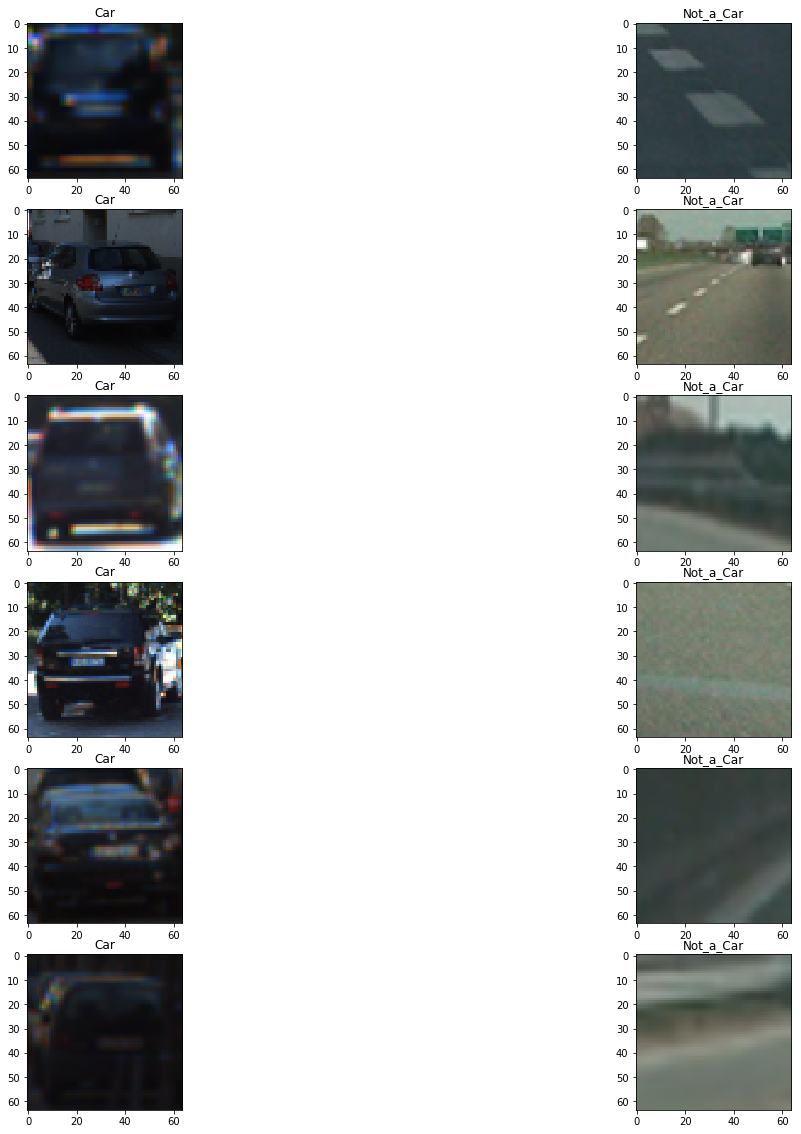
The code for this step is contained in the first code cell 24 of the IPython notebook. I started by reading in all the vehicle and non-vehicle images. Here is an example of one of each of the vehicle and non-vehicle classes:

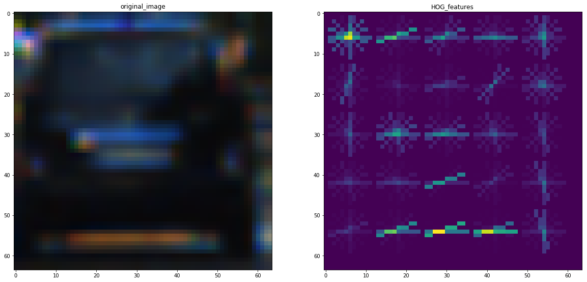
I then explored different color spaces and different skimage.hog() parameters (orientations, pixels_per_cell, and cells_per_block). I grabbed random images and displayed them to get a feel for what the skimage.hog() output looks like.

Here is an example using the Gray image and HOG parameters of orientations=8, pixels_per_cell=(8, 8) and cells_per_block=(2, 2):

####2. Choice of HOG parameters.

I tried various combinations of parameters for orientation, pixel_per_cell but kept cell_per_block constant at (2,2) and tried expermenting with SVM and RandomForest classifier to check thier accuracy. I got the maximum accuracy with pixel per cell at (8,8) and oreintation at 8

####3. Training a classifier using your selected HOG features and color features (cell 36).

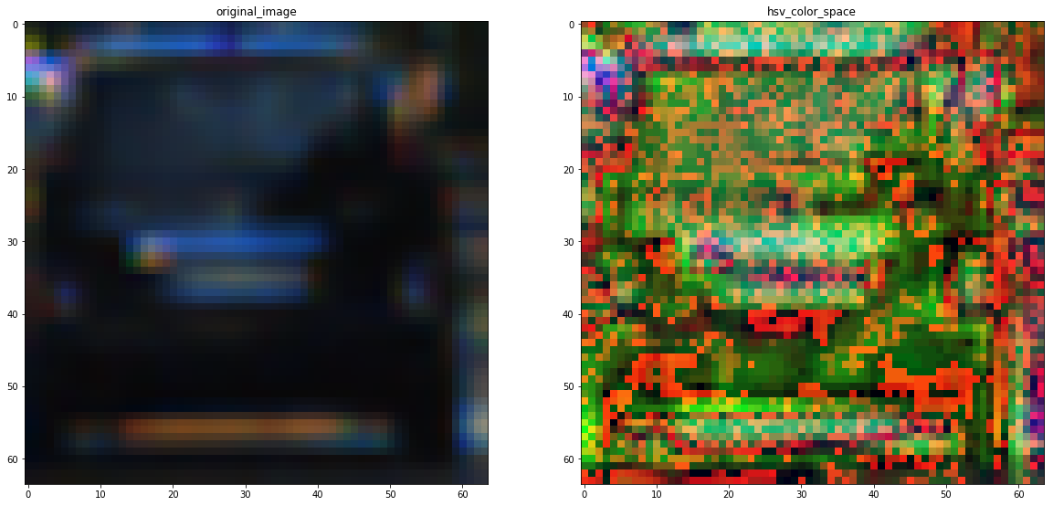
With Hog features, I also used HSV colorspace spatial fetaures as shown below

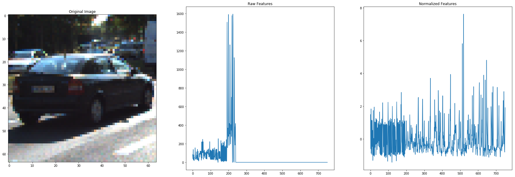
and also histogram features in HSV and RGB colorspace using 8 bins for each channel. I normalized all the features as shown below to avoid bias in weights.

I trained a linear SVM and Random Forest using this normalized data. The best accuracy of the classifier were:

1. SVM : 0.981981981982
2. Random Forest : 0.989301801802 So I choose to go forward with Randomforest

Sliding Window Search

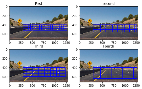
####1. sliding window search. (cell 42) I tried to scale the window in four sizes, to detect car near as well as far way. The four scales are shown below Scales = ( 1, 1.25, 1.5, 1.75 ) The range of window size was from (80,160) while the region searched was x in (300,1280) while y in (400,700) Please see the four scale in the image below !

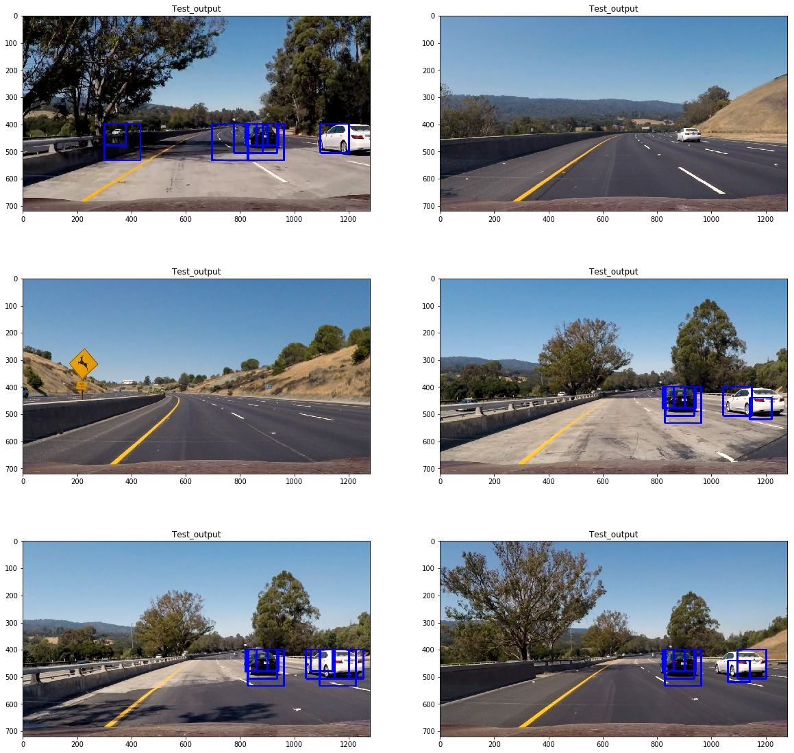
####2. test images to demonstrate how pipeline is working.
With Hog features, I also used HSV colorspace spatial fetaures as shown below and also histogram features in HSV and RGB colorspace using 8 bins for each channel.I normalized all the features to avoid bias in weights. Please see the below image to see the results.

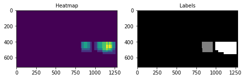
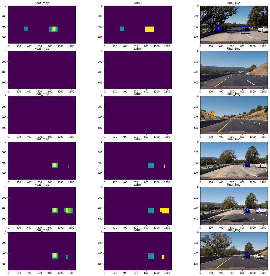
Heat Maps (Cell 53):

I created heatmaps based upon the prediction of the classifier to avoid overlapping windows and false positive as shown in lecture. I recorded the positions of positive detections in each frame of the video. From the positive detections I created a heatmap and then thresholded that map to identify vehicle positions. I then used scipy.ndimage.measurements.label() to identify individual blobs in the heatmap. I then assumed each blob corresponded to a vehicle. I constructed bounding boxes to cover the area of each blob detected. The high probability of finding a car was found using thresholding this heatmap.

Heatmaps:

Final_test_image

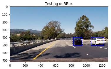
###Here the resulting bounding boxes are drawn onto the last frame in the series:

Here is the output of scipy.ndimage.measurements.label() on the integrated heatmap from all six frames:

Video Implementation

####1. Final video output.
Here’s a link to my video result

###Discussion

####1. Briefly discuss any problems / issues you faced in your implementation of this project. Where will your pipeline likely fail? What could you do to make it more robust?

1. The window search technique can be improved by using probabisitic distribution which could reduce the latency of the pipeline
2. The sclaing of the window need to set correctly to get accurate result. Could be improved by ising dynamic scaling once a vehicle is detected.
3. Different sclaing in X and Y may also provide good results as car shapes are flat.